5th order constant coefficient example

Let's compare standard collocation with preconditioned collocation. We take a fifth order example with constant coefficients,

$u^{(5)}(x) + u^{(4)}(x) - u'(x) - u(x) = f(x),$

with $u(x) = \sin(x^2)$ . The right hand side function for this problem is

$f(x) = ( 16 x^4 + 160 x^3 - 13 ) \sin(x^2) + (32 x^5 - 48 x^2 - 122 x) \cos(x^2).$

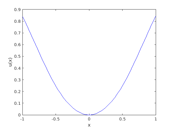
m = 5;
N = 64;
[Dm,x] = chebdifmat(N,m,1);
Uexact = sin(x.^2);
f = @(x) (16*x.^4 + 160*x.^3 - 13).*sin(x.^2) +...
    (32*x.^5 - 48*x.^2 - 122*x).*cos(x.^2);
plot(x,Uexact,'b')
xlabel('x')
ylabel('u(x)')

Next we need to add boundary conditions to the problem. We'll use Dirichlet and Neumann at both 1 and -1, as well as a condition on the second derivative at 1.

BC = [ Uexact(1) ; 2*cos(1) ; 2*cos(1)-4*sin(1) ; Uexact(end) ; -2*cos(-1) ];

The first three conditions are at x=1, while the last two are at x=-1. We store this information in two rectangular matrices, for use with the PSIM later.

U1 = eye(3,5); U2 = eye(2,5);

Now it's time to decide on the row removal. Which rows will we take off to replace with boundary conditions? This choice is necessary to construct a square PSIM. We'll choose the rows symmetrically: the first and last two rows, as well as the middle row.

v = [1 2 N/2+1 N N+1];

We're now ready to construct the operators. We start with the differential operator.

I = eye(N+1);
A = Dm(:,:,5) + Dm(:,:,4) - Dm(:,:,1) - I;

Replace those rows chosen for removal with boundary conditions.

A(v,:) = [ I(1,:) ; Dm(1,:,1) ; Dm(1,:,2) ; I(end,:) ; Dm(end,:,1) ];

Now build the right hand side, replacing those elements associated with the removed rows with the boundary condition values.

F = f(x); F(v) = BC;

Lastly, we construct the pieces needed to use the PSIM. There is the portion of the linear operator that is not inverted by the PSIM.

Atail = Dm(:,:,4) - Dm(:,:,1) - I; Atail(v,:) = 0;

Then there is the PSIM itself.

B = PSIM(N,m,v,U1,U2);

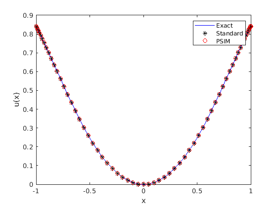
And now we solve the systems and present the results.

UA = A \ F;
UB = (I + B*Atail) \ B*F;
plot(x,Uexact,'b',x,UA,'k*',x,UB,'ro')
xlabel('x')
ylabel('u(x)')
legend('Exact','Standard','PSIM')